
In this chapter, we are going to learn how you can create and add measures and use them in your visualizations. We’ll learn how to add simple aggregation measures based on a single field as a custom field, and then we will dive into the LookML code and write measures that will be added directly as fields to your view.
Finally, we’ll learn how to use Looker’s SQL Runner to write and run SQL queries, make a derived table from an existing one, and add it to a project. Use LookML for reusable business definitions; SQL Runner is useful for testing SQL and developing derived tables. LookML also generates SQL, so writing SQL directly is not automatically slower or faster.
For our use cases we are going to use an example dataset of Worldometer Coronavirus Daily Data. You can learn from the following examples and implement them with your own data. The original screenshots are from the 2022 tutorial and show the classic Looker interface and historical sample data. New real Looker captures are labelled separately and use synthetic teaching data; labels and layout may differ in your instance. This chapter covers Looker, not Looker Studio.
Before you start, you need a working BigQuery connection, a project and an Explore for this table, and permission to edit the dashboard. Custom fields require the appropriate custom-field permissions; editing LookML requires developer access, and SQL Runner requires use_sql_runner. Work in Development Mode when changing LookML.

Adding simple measures
To start off, we’ll learn how you can add basic measures of aggregations like sum, average, min and max as a custom field to your Explore while making a dashboard tile, without writing LookML.
I prepared a dashboard to work with, created a connection to BigQuery where our dataset is, and created a project with this connection. We learned to do all of these in the previous chapters.
Start by editing the dashboard and adding a new visualization tile (Add → Visualization). Select the Explore you want (in this example, Worldometer Coronavirus Daily Data under Yuval Project 2).

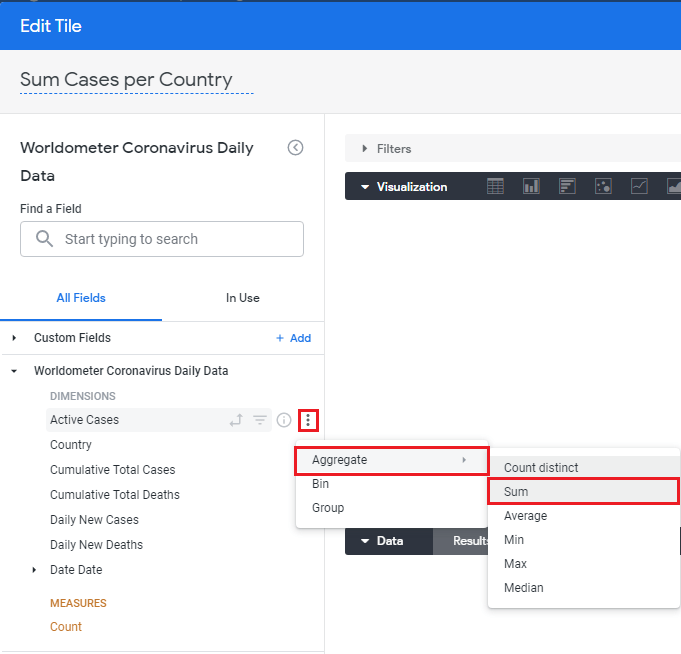
Looker allows us to create simple measures for numerical data fields by clicking the three-dot More menu next to the field, selecting Aggregate, and choosing the calculation. In this case, for the Active Cases dimension select Sum.
 (opens in a new tab)
The measure Sum of Active Cases is now added under Custom Fields. The available aggregations depend on the field type; for a string such as Country, the classic menu offers Count distinct and List of unique values. In newer Explores you can also use Custom Fields → + Add → Custom Measure in the Configure panel.
 (opens in a new tab)
Now add the Country dimension and click Run. For an active-case snapshot by country, first filter Date to one specific date shared by the countries you want to compare. Summing Active Cases across multiple dates counts repeated daily observations, not distinct people or total infections. The original all-date totals should not be presented as current active cases. Save the tile and the dashboard when ready.
Writing measures in LookML
In many cases, we’ll want calculations beyond an ad hoc custom measure, or we’ll want to make a definition reusable. We can write those measures in LookML.
Going back to our coronavirus example, open the Explore and select Go to LookML. If you do not have developer access, ask your Looker developer to add the measure.

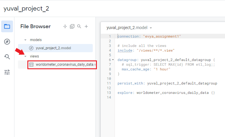
In Development Mode, open the view where you want to add the measure by expanding views and selecting worldometer_coronavirus_daily_data.
 (opens in a new tab)
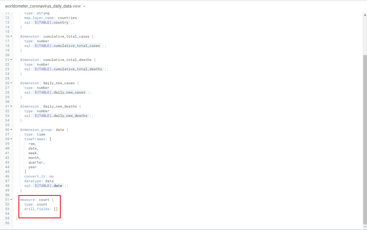
As we talked about in the second chapter, this is where you see the LookML of your view’s fields: dimensions and measures. By scrolling down, you’ll get to the default count measure and any other measures.
 (opens in a new tab)
As an example, let’s create a measure that returns the country name that sorts last. Give it the name max_alphabet_country, set its type to string, and write the aggregation explicitly in its SQL:
measure: max_alphabet_country {
  type: string
  sql: MAX(${country}) ;;
}
The string type does not add an aggregation itself; MAX() supplies it here. The result follows the database’s string ordering and the query’s filters and groups. A drill_fields setting controls which fields appear when drilling into a measure; it is not specific to dates. It is not needed for this example. Remember to end the SQL expression with double semicolons.
Click Save Changes, validate the LookML, and reopen or refresh the Explore in Development Mode. The new field should appear under Measures. Saving in Development Mode does not make changes available to production users; follow your project’s commit and deployment process after testing.

Try it by selecting the measure and pressing Run. In the original sample, without Country selected as a grouping dimension, the result was Zimbabwe. Your result depends on the data, filters and string ordering.
 (opens in a new tab)
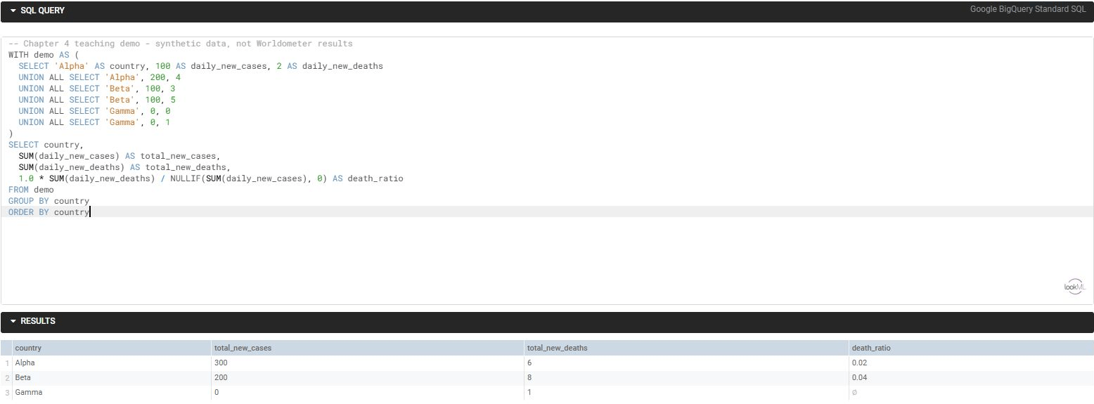
Let’s walk through another example. This time we’ll create a measure based on more than one field. For this dataset, we’ll divide the sum of Daily New Deaths by the sum of Daily New Cases over the selected rows.

This is a ratio of reported deaths to reported cases for the selected period, not a patient-level fatality rate: deaths and reported cases can refer to different cohorts and reporting dates. Reporting adjustments and negative daily values can also affect the result.
First define two aggregate measures, then use a type: number measure to divide them. Add these definitions inside the existing view, reusing existing equivalent measures if they are already present:
measure: total_new_cases {
type: sum
sql: ${daily_new_cases} ;;
}
measure: total_new_deaths {
type: sum
sql: ${daily_new_deaths} ;;
}
measure: death_ratio {
type: number
label: "Reported Deaths / Reported Cases"
sql: 1.0 * ${total_new_deaths} / NULLIF(${total_new_cases}, 0) ;;
value_format_name: percent_2
} (opens in a new tab)
NULLIF(..., 0) changes a zero denominator to NULL, avoiding division by zero. The result remains NULL when the denominator is zero. The percentage format displays a ratio such as 0.02 as 2.00%; do not multiply the SQL result by 100 as well.
A type: number measure does not aggregate raw dimensions for you. Referencing aggregate measures makes this calculation work at the grouping level selected in the Explore. Select Country, filter the date range, select Reported Deaths / Reported Cases, and click Run. You do not need to select the two component dimensions or hide them from the visualization. Adding raw dimensions would change the query grain rather than fix the aggregate definition.
 (opens in a new tab)
Save and validate the changes, then test in Development Mode. Check zero-denominator behavior and compare a few countries against an independent aggregation before deploying.
Working with SQL in Looker
In some cases you may want to work directly with SQL in Looker. For example, you can take the SQL generated by an Explore and use it as a starting point for a window-function ranking and a derived table.
Open the Explore’s SQL tab in the Data panel and select Open in SQL Runner.
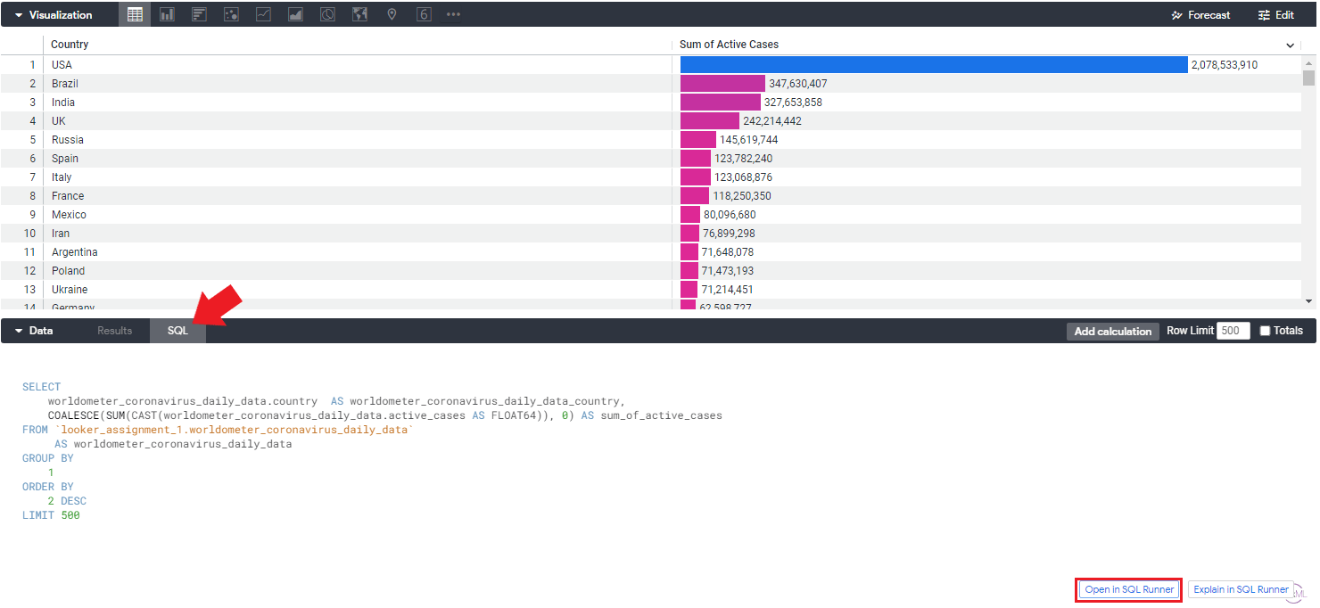 (opens in a new tab)
SQL Runner provides an editor where you can query the database connection directly. Verify the selected connection and BigQuery project/dataset. SQL Runner queries do not automatically inherit LookML access filters or other model logic, so use only data you are authorized to query.
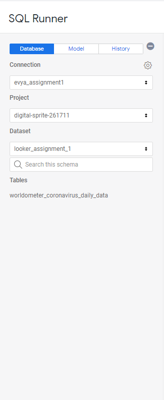
For this example, rank countries by their active-case count on the latest date available anywhere in the table. This compares one shared date, instead of adding snapshots across time. A country without a row for that date is absent from the result. Replace the fully qualified table path below with your own project, dataset and table:
WITH country_snapshot AS (
  SELECT
    country,
    SUM(active_cases) AS active_cases_snapshot
  FROM `YOUR_PROJECT.YOUR_DATASET.worldometer_coronavirus_daily_data`
  WHERE date = (
    SELECT MAX(date)
    FROM `YOUR_PROJECT.YOUR_DATASET.worldometer_coronavirus_daily_data`
  )
  GROUP BY country
)
SELECT
  country,
  active_cases_snapshot,
  RANK() OVER (ORDER BY active_cases_snapshot DESC) AS active_cases_rank
FROM country_snapshot
Click Run to check the results. RANK() gives tied values the same rank and leaves gaps afterward. This example ranks the whole result; use PARTITION BY only if you need a separate ranking within groups. To display rows in rank order, sort by the rank field in the Explore or add an outer ORDER BY active_cases_rank, country when testing the standalone SQL.
 (opens in a new tab)
Remove an inherited LIMIT from the SQL before turning it into a derived table, unless limiting the table is intentional. Otherwise the derived table may silently omit countries. Check any inherited filters too. A filter applied later in an Explore does not automatically recompute a rank already calculated inside this SQL; this example always uses the table’s latest date.
Once the results are correct, open the SQL Runner gear menu and select Add to Project. You can also use Get Derived Table LookML to copy the generated definition manually.

Select the project (in the original example, yuval_project_2) and enter a view name. We’ll use sum_of_cases_per_country_ranked to keep the original example’s view name. Click Add. This creates a LookML view containing a derived-table definition; it does not by itself create a permanent database table.
 (opens in a new tab)
Place the view under views if that is where your model’s include pattern expects it, or update the include pattern to match its location. Moving files is a project-organization choice, not a requirement for every model.

Check the generated dimensions against the SQL output: country, active_cases_snapshot and active_cases_rank. Because this query groups by country, Country can be the primary key only after you verify that every country value is non-NULL and unique. Do not use rank as the primary key: tied values can share a rank.
Now open your project’s model file, ensure it includes the new view, and add an Explore:
# Use this pattern if view files are stored under views/.
# Keep an existing include if it already covers the new view.
include: "/views/**/*.view.lkml"
explore: sum_of_cases_per_country_ranked {}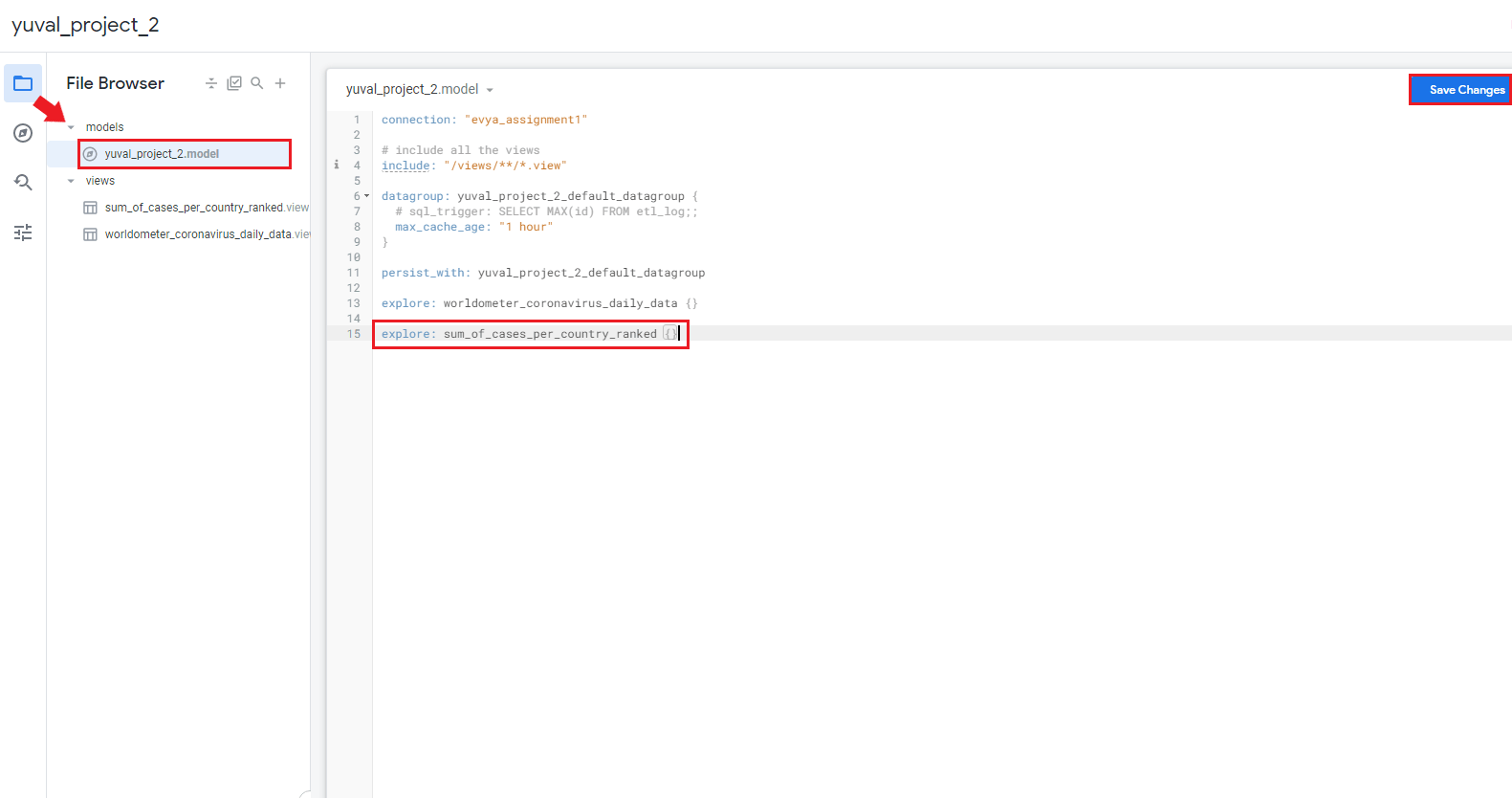 (opens in a new tab)
Save Changes, validate LookML and test the new Explore in Development Mode. Select Country, Active Cases Snapshot and Active Cases Rank, then sort by rank. Follow your project’s normal commit and deployment process to make the tested Explore available in production and add its visualization to a dashboard. A derived table is not automatically persistent; persistence needs separate configuration.
That’s all for this chapter.