In this chapter, we are going to build a dashboard based on Looker’s demo product data. We’ll learn how to create a dashboard, what Tiles are, what you can do with them and how to add them to your dashboard.
In addition, we will make some example graphs while covering many useful features and use cases you can implement in Looker.
Finally, we will go over some adjustments you can make to your dashboard such as adding filters to it, and automatically refreshing your graphs while the dashboard is open to keep the displayed results up to date.
Before you begin: This chapter uses the original eCommerce sample model, including Orders, Items and Users, Share of Wallet Analysis and Affinity Analysis. You need access to those Explores and permission to create and edit dashboards in a suitable folder. An administrator or model developer can provide a suitable sample model. The screenshots are original sample-data examples; their values and dates are not live results. They illustrate the classic dashboard tile editor; labels and styling can vary by enabled interface.
Creating a Dashboard
Dashboards are visual displays of our data.
- To create one, first log in and open a folder where you have permission to save dashboards.
- Press on the New button that appears on the top right corner of your screen and Select Dashboard.
 (opens in a new tab)
- Give a name to the dashboard, and after that Press Create Dashboard
 (opens in a new tab)
Adding Tiles and Visualization Use Cases
At first, our dashboard is empty: we haven’t add anything to it yet…
- Click on Edit Dashboard
 (opens in a new tab)
This is where you edit your dashboard and add graphs and visual data to it.
In Looker, a dashboard is made of “Tiles”, blocks, that each is a component in the dashboard, such as a Visualization (Graph, Numerical data) or a Text Tile (notes, subtitles…)
- Let’s add a tile. Click on Add, then Select Visualization
- We will choose the sample Orders, Items and Users Explore. The sample eCommerce model must already be available in your Looker instance; these Explores are not automatically included in every instance.
- Press on Orders Items and Users.

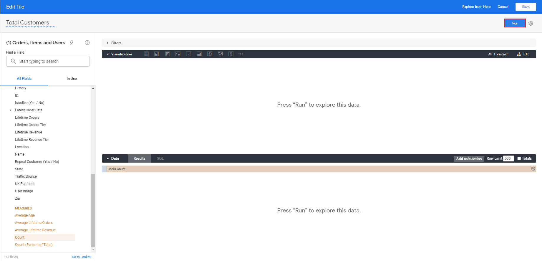
- For this example, Give your Tile the title of “Total Customers”.
- Select the Users view.
 (opens in a new tab)
- From the Users list of fields, scroll down to MEASURES and select Count.
 (opens in a new tab)
- Press Run (appears on the top right corner of your screen).
 (opens in a new tab)
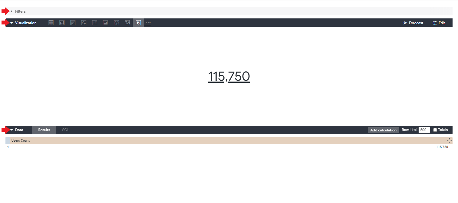
You should now get the number of Users.
The original tile title “Total Customers” refers to the Users Count measure in this example. Check the model’s count definition before treating it as a count of paying customers. With the date filter added later, the result is further restricted by the mapped order-item creation date.
- Notice that there are three different sections: Filters,Visualization and Data:
Filters: the “Filters” section is where you can create filters for your queries.
Visualization: the “Visualization” section is where you can see how it will be added to your Tile.
Data: the “Data” section is where you can see the data in its tabular form under Results, and the actual SQL behind it under SQL.
 (opens in a new tab)
- Click the Save button on the top right corner of your screen.

The Tile of total customers is now added to your dashboard.
We want the dashboard to be neat and conveniently designed for our clients. You can improve the design by adding notes and texts to your dashboard .
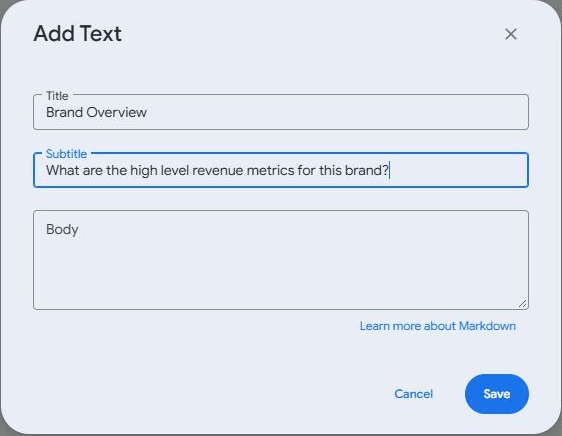
- Press the Add button and select Markdown to use the title, subtitle and body workflow below.

In the current menu, choose Markdown. Its title/subtitle/body dialog is still titled “Add Text”.
- Inside the Title and Subtitle panes, copy and enter the following text:
Title: Brand Overview
Subtitle: What are the high level revenue metrics for this brand?
Click Save.
 (opens in a new tab)
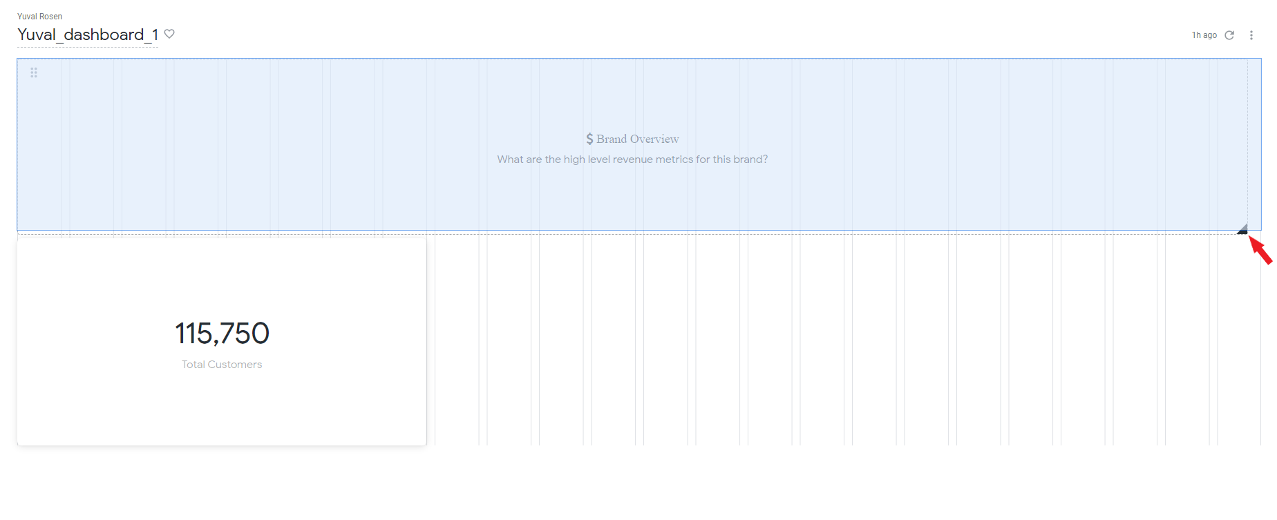
- Now that this Text Tile is added to your dashboard, drag the Tile of total customers below the Text Tile by pressing and holding the dragging button on the top left corner of the Tile:
 (opens in a new tab)
- Use the “black triangle” button on the bottom right corner of the Text Tile to widen it. Text alignment is controlled by the text tile’s formatting, rather than by resizing it.
 (opens in a new tab)
- For each new Tile you create, or change you make in your dashboard make sure to save it right away by pressing the Save button on the top right corner of your screen!
Save your dashboard edits before leaving edit mode.
 (opens in a new tab)
- After saving you will be back to the visualization mode so go back to editing mode by clicking on the “three dots menu” button on the top right corner of your screen and selecting Edit dashboard, or by pressing ctrl+shift+e
 (opens in a new tab)
Let’s add another Numerical data bullet to our dashboard.
- Press Add and select Visualization
- Select the Orders Items and Users explore.
This time the number we want to display is the average price at which a item is sold
Click on Order Items

- From the list, select the measure Average Sale Price and press Run

You should now get the average sale price.
Average Sale Price is an item-level average. It is not average order value, which requires an order-level definition such as total order revenue divided by the number of orders.
- Don’t forget to give your Tile a title from which it will be possible for anyone to understand what the Tile is about. In this example, name it “Average Sale Price”.
Choose the Single Value visualization if needed, then click Save to add this tile.
Now, let’s add a graph to our dashboard:
We are going to make a graph of two trend lines, one for the average sell price and one for the total sell price by dates, so there will be two different Y-axes, and the X-axis will be based on Dates.
- Press Add and select Visualization
- Once again Choose Orders Items and Users, then Press Order Items, then from Created Date, Select Date.

Now for the vertical axes: one will show total sales value, and one will show average sale price.
- Scroll down to MEASURES and Select Average Sale Price.
- For our second Y-axis Click on Total Sale Price.
 (opens in a new tab)
- Notice that you can drag and switch position between fields to change the visual order, for example, place Total Sale Price before Average Sale Price. Assign the axes explicitly in the visualization settings below.
 (opens in a new tab)
- Don’t forget to give the graph a suiting title that expresses what it is about .
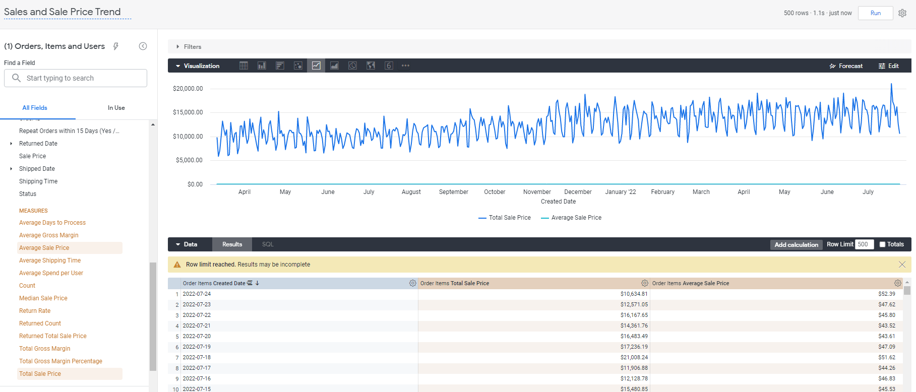
- Press Run, and you should get the following graph:
Choose the Line visualization if it is not already selected. If you see “Row limit reached”, narrow the date range or use an appropriate row limit and rerun before interpreting the chart as a complete time series.
 (opens in a new tab)
We got a graph with a horizontal axis of dates as wanted.
However, it’s inconvenient for the user: we got a single Y-axis of prices in the scale of the Total Sale Price field prices caused by the fact that both Total Sale and Average Sale are fields of prices and there are big gaps between the prices of the fields as well so you can barely see the fluctuations in the Average Sale line…
We need to manually change the graph so it will have separated Y-axes for each field of prices.
- To do so, on the visualization tab, press the Edit button and select Y.
- You can see that both of the fields are under Left 1, so simply drag one of them below the Right Axes section.
 (opens in a new tab)
Now that the graph has two y-axes as we wanted, we can make it even more convenient by removing the unnecessary decimal format of the numbers of the y-axes, as a display choice for these currency axes. Decimal precision is independent of whether a value is a percentage.
- You can change the format by scrolling down to Y Axis Format and entering the format you want. In our case enter: “$##,###”

- You need to edit each of the axes separately. We applied this format change only on our left one, so under the Configure Axes select Right 1 and do the same to change its format as well.

The graph now looks much better than it did at the beginning and meets our needs!
- Click Save, then move and/or resize the Tiles to design your dashboard if you’d like and then click Save again, this time to save the dashboard itself and return to view mode. To continue editing, choose Dashboard actions → Edit dashboard
 (opens in a new tab)
For the next example, let’s say we are a clothing store and we want to see how much is the total sell price of each product categories, for each department (men and women).
For that, we will make another graph, of total sell price by category and department.
- Just like before, press Add and select Visualization, then choose Orders Items and Users. (Give the tile a suiting title such as “Most Popular Categories”)
- From Order Items select Total Sale Price, and from Products select Category .
Here, “Most Popular Categories” means categories ranked by Total Sale Price (sales value), rather than by item count.
 (opens in a new tab)
- Pressing Run will get us the following bar chart.
* Notice that you are able to change the visualization type by choosing a different kind on the visualization tab. Stick with the bar format for this graph, though.
 (opens in a new tab)
In order to make the total price be displayed for each department, we need to add a secondary dimension.
- From Products press the Pivot data button of the Department dimension to make each value in the dimension become a column in the graph.
- Press Run to see the result.

We got the desired graph, however we can make it look even better.
- Click the visualization section’s Edit button, then from the Plot tab, under Series Positioning, select Stacked.
 (opens in a new tab)
- The graph now presents the total price of each category divided by men and women, ordered descending by the total sale price of men for each category. In order to make it more convenient and organized, Let’s make it ordered by the general total sale price of each category. Doing so requires us to add another field that will be this general total: a scheme of the total amount for women and men.
- Check the Row Totals box that appears on the Data section and press Run.
 (opens in a new tab)
A Total field is now added under the Data section with the scheme of total sale price for men and women values.
- Now we can make the graph ordered descending by this total value by clicking under its name on the Order Items Total Sale Price field in the Data section, so an arrow pointing down will appear next to it.
 (opens in a new tab)
- Our graph is ready. Make sure to save it and then save the dashboard itself.
Afterwards, go back to editing mode (Edit dashboard).
For our next use case we’ll make a line chart and add a filter to it.
- As you must know how to do it by now, add a new Visualization Tile (Add->Visualization), but this time select a different explore: Share of Wallet Analysis.

Give it the title “Brand Share of Wallet over Customer Lifetime”. That is what our graph is going to be about.
Let’s limit the chart to Months Since Signup values of 18 or less. Check the definition of this field in your sample model: it may measure elapsed time at an order rather than the user’s age as of today.
From Orders press the “Filter by field” button of the Months Since Signup dimension.
 (opens in a new tab)
- Set the filter to “is less than or equal to” and enter the number of months that the condition is relative to (18 in our case).
* After you filtered it, click the dimension itself to make sure it’s added as a field under the Data section.
 (opens in a new tab)
Now let’s add the measures:
- From the Share of Wallet (Brand Level) view, select Brand Share of Wallet Within Company and Total Sales – This Brand

- Press Run.
- Change the type of the graph to Line on the Visualization tab.
Add Months Since Signup as the dimension, and review the share measure’s definition and numeric format in your model. Place the share measure on its own percentage axis and Total Sales – This Brand on a currency axis, using the Y-axis settings shown above. A shared currency scale can flatten the share series and make the chart misleading.
 (opens in a new tab)
* Don’t forget to save the tile and then the dashboard itself when you are done. Then go back to editing mode.
- For our last use case, once again add a visualization tile and this time select the Affinity Analysis explore .

- Give it the title of “Purchasers of This Brand Also Bought (Brand Affinity)”.
* Notice that this explore has a required filter set by default for the Affinity Product B ID dimension: whoever wrote the LookML code for this explore defined it that way. - Add another filter to the tile for the Affinity Score (by Order Basket) measure that is under the Affinity field, by clicking on the “Filter by field” button next to it, and just like the other filter set it to “is not null”.
 (opens in a new tab)
- Now, click on this measure itself to add it as a parameter to the graph and additionally, select the Affinity Score (by User History) and Combined Affinity measures as well.

- Select the Brand dimension under the Product A Details and Product B Details fields.

- Press Run, and change the visualization type to Table.
 (opens in a new tab)
Let’s say we don’t want to present the Product A brand in our visual data, but we still want to make calculations with it for other fields like measures that depend on this field, so it will still remain in the Results tab of the Data section and only visually not be shown.
- To do so, press the cogwheel button next to the “Product A Details Brand” fields under the Data section, and select Hide from visualization.
 (opens in a new tab)
Order by the Combined Affinity measure by clicking it, under the Data section.

We only added it so we can order the data by it, however we don’t want it as a column in our visual table in the tile itself.
Just like we learned how to do before, press the cogwheel button next to this measure and click on Hide from visualization.

You can add colors beyond the numbers to present them, to the Affinity Score (by User History) column in the table, just like the Affinity Score (by Order Basket) column has.
- Press the Edit button on the visualization toolbar, select Series, click on the desired column name (Affinity Affinity Score (by User History)), and turn on Cell Visualization.

You can choose the set of colors you’d like to use and even custom an original set.
 (opens in a new tab)
To sum it up, in the table we got, in the visual layer we don’t present the Brand of Product A details, and the Combined Affinity measure, but we do base our data and calculations on those fields and that’s why we add them to the Data section’s Results: the measures are grouped by both brands A and B, and the data shown is ordered by the Combined Affinity measure.
 (opens in a new tab)
- Save the tile.
- Play around with the tiles’ positions and sizes to design the dashboard, and don’t forget to save it when you are done.
 (opens in a new tab)
Dashboard Filters
Dashboard filters let us narrow a dashboard’s results to only the we are interested in, affecting all
the tiles (it is possible to apply the filter to only one dashboard tile).
- To add one, in editing mode, click Filters and then select Add Filter.

You will now see the list of Explores that are used in your dashboard.
Let’s make a Generic date-based filter.
- In the search pane, enter “date”.
- From Orders, Items and Users, under Order Items, under Created Date select Created Date.
After selecting the field, click Add to open its filter settings.
 (opens in a new tab)
- Change the filter’s title to “Date”.
Now we need to set a default dates range that the data will be filtered on. Later on, a viewer of our dashboard will be able to temporarily change the range value for his needs (without affecting the dashboard for other viewers and users).
- For Control select Advanced. It will give us and the future viewers of the dashboard lots of options and freedom to filter.
- For our example, under Configure Default Value select is in the last, enter 90, and select days. The tiles mapped to this filter will query the last 90 days. This is a rolling day window, not exactly three calendar months. For a static sample dataset, choose a date range that contains records.
Use Advanced in the Control menu; this is separate from the Advanced toggle beside the Filter by search field.
 (opens in a new tab)
In Tiles To Update, review the Field to Filter for every tile. Tiles based on the same Explore are normally mapped automatically. For tiles from another Explore, select the corresponding field manually or choose Do Not Filter.
Go to Tiles to Update, and from the list of our visualization tiles, for the Brand Share of Wallet over Customer Lifetime tile, change the Field to Filter: under Share of Wallet Analysis, below Order Items, select Created Date.

Use a field with a compatible date type and the same business meaning. A matching type alone does not make two date fields equivalent.
- For the “Purchasers of This Brand Also Bought (Brand Affinity)” tile, there isn’t a Created Date filed in its explore so in the Field to filter select Do Not Filter.

- The filter is ready. Click Add.
- Press on Update and save the dashboard.
 (opens in a new tab)
You can change the filter date range even in visualization mode by pressing and editing it and then clicking on the update button. See how the data changes according to the changes you make to the filter.
 (opens in a new tab)
Automatically Refreshing the Dashboard
Looker can automatically refresh dashboard results while the dashboard is open in the browser. This is not a background query schedule; automatic refreshing pauses in edit mode.
*Notice that any such update means querying the data, so take into consideration the cost matter before applying such thing.
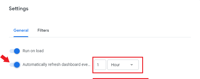
- In order to automatically refresh your dashboard, go to editing mode (Edit Dashboard) and press on Settings.

- In General, turn on Automatically refresh dashboard, and then enter the period of time you want for it to update.
- You are able to separately choose different period of times for each tile in the dashboard to update by changing the Refresh frequency for the tiles you want.
- If you want to apply this, press Save, otherwise just cancel.
Automatic refresh bypasses Looker’s cache and can send new database queries. Choose an interval appropriate to the data and query cost; refreshing the dashboard does not load new data into the database.
 (opens in a new tab)
This wraps up this chapter.